Introduction to SAP HANA Modeling

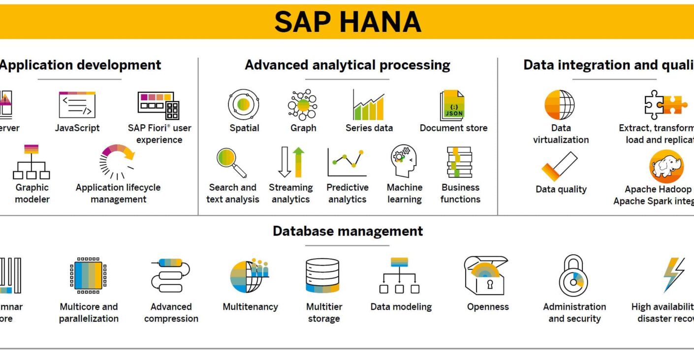
SAP HANA Overview

SAP HANA is a combination of HANA Database, Data Modeling, HANA Administration and Data Provisioning in one single suite. In SAP HANA, HANA stands for High-Performance Analytic Appliance.

“SAP HANA Information Modeler also known as HANA Data Modeler is the heart of HANA System enabling you to create modeling views at the top of database tables and implement business logic to create a meaningful report for analysis.”

.

Most of the SAP HANA’s applications are based on HANA Modeling. So let’s start with the basic understanding of 3 layers of SAP. As per the Traditional Approach, the role of the database is to just provide data. According to the SAP architecture, there are three layers:

• Presentation Layer
• Application layer
• Database layer

The application layer sends various business-scenario select queries to the database layer to fetch the data. Further, the raw data is sent from the database to the application. The application layer processes the data by filtering it, performing aggregation, and doing calculations. Here, the bulk of data gets transferred from the database to the application layer, and the application layer performs all complex work.

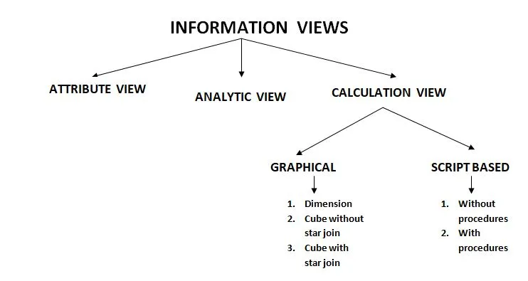
Now, as per the HANA approach, the thumb rule is to perform maximum work in the database layer. For this scenario, a modeling layer is built on top of the database layer, and it provides simply the result to the application layer. With SAP HANA, one can build Information views to perform various tasks according to business requirements such as applying filters to data, performing calculations, applying conditions. For this reason, HANA Modeling views include Information Views which further include Attribute view, Analytic View, and Calculation view.

The following are the advantages of using SAP HANA Modeling:

• There is no performance degradation
• No transfer of data
• No-load on the application layer, since it will just get the result set from the database layer
• Information views can be reused

SAP HANA Information Views

Now let’s dive into the Information views and learn more about them. The following are some key terms that are used frequently while creating Information views:

• Measure: A numeric value on which arithmetic operations can be done such as sum, count, max, min average is called a measure. Examples are the net amount, gross amount, number of products sold
• Attribute: Elements that describe the quality of the measure. Examples are Customer name, vendor name, date of creation, product id, country, currency
• Dimension: Grouping of similar attributes together for better analyzing of a measure is called Dimension. For example, Dimension 1 consists of all data of customers, Dimension 2 consists of all data of products and so on
• Fact table: The fact table consists of measures or keys used to identify each dimension table
• Star join: Star join consists of one fact table surrounded by all dimension tables

Below is the segregation of the Information views:

Attribute View:

1. Attribute views are created on top of Dimension tables.
2. It can be created using single or multiple tables or also other existing attribute views.
3. These views are preferred when there are no measures or no calculations to be performed.
4. Also, these views can not be consumed in reports, so there use is very limited. attribute views can be used purely in Analytic views or Calculation views.
5. Since there is an option of Calculation view of type Dimension, the Attribute view is depreciated up to a certain extent.

Analytic View:

1. Analytic views are based on star join or star schema, where the fact table also called Data foundation are surrounded by Dimension tables.
2. The dimension table contains the descriptive data and the fact table consists of both descriptive data and measurable data.
3. Analytic views are used when we require aggregated data from the tables.
4. Since there is an option of Calculation view of type cube, the Analytic view is depreciated up to a certain extent.

Calculation view:

Calculation views can perform complex calculations that are not possible with other views. As seen before, calculation views are of two types: Graphical and SQL script-based.

• Dimension: Dimension Calculation view is similar to the Attribute view. It cannot handle measures. Every column is always treated as an Attribute. The default upper node of this type is the Projection node.
• Cube without star join: Here we will be using normal attribute views and analytic views. The default upper node is Aggregation.
• Cube with star join: You can not use Column tables, Attribute views, or Analytic views in star join. The advantage of using a star join is its simplicity. The default upper node in this type is the star join

Creating an Attribute View in SAP HANA

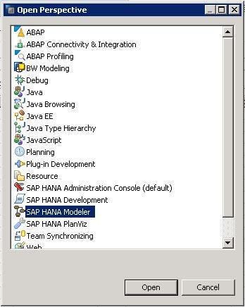
We need to set the perspective to get access to these views. For that, navigate and click on the open perspective icon. Search for SAP HANA MODELER.

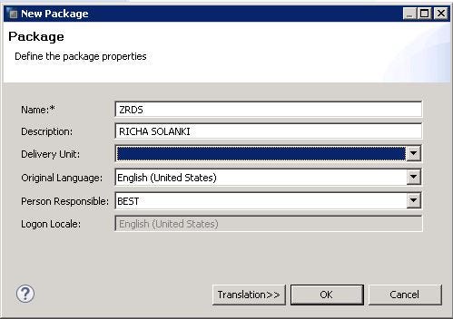
Once the screen gets loaded, towards the left panel, click on the catalog and check for the existing schema (table which you want to work on). Here we are using the DHK_SCHEMA table for the Attribute view. All the artifacts are created under the content folder inside the custom package. So to create a custom package, right-click on the content ->Package. Provide the name along with the description.

NOTE: All the ‘z’ package which you will create, will come at the end.

Under the custom package,

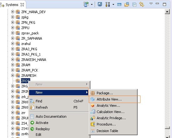
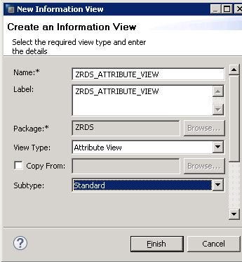
Enter the Attribute view name and click on Finish.

Once you click on the finish button, the following Information View screen will be displayed.

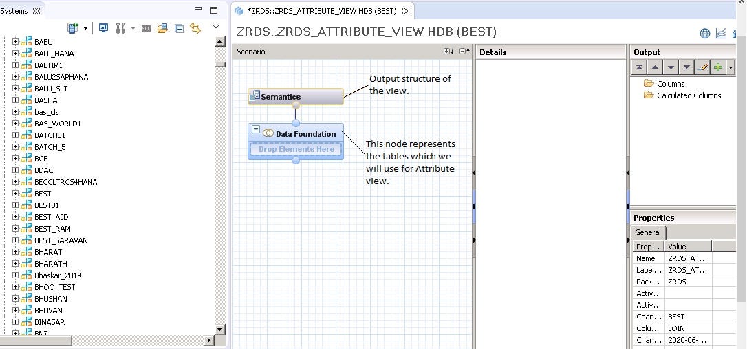
• The left panel is the hierarchy of all the tables, views that we have to use to create the Attribute view.
• Semantics — This node is responsible for the output structure of the created view.
• Data foundation — This node is a collection of tables which we will use to create an Attribute view. (Drag and drop is allowed).

Let’s create our first Attribute View.

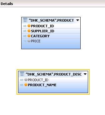
• Navigate to DHK_SCHEMA. Further under the table node, we will work on two tables namely ‘PRODUCT’ AND ‘PRODUCT_DESC’.
• Drag ‘PRODUCT’ and ‘PRODUCT_DESC’ tables one by one and drop into the data foundation node.

• Now we need to select the fields which we want to see in our view. Hence, select the bullet fields in the Details panel. When you select, the color of the bullet will change from grey to orange indicating the field is been selected.

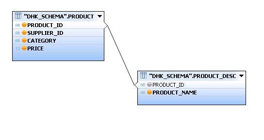
• Now, connect the PRODUCT_ID field of table ‘PRODUCT’ to the ‘PRODUCT_ID’ field of table ‘PRODUCT_DESC’ to perform join.

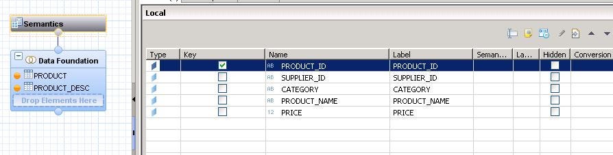
• Further, click the Semantics node. The list of the fields which we want to see in the attribute view will be displayed. Select the checkbox to mark the field as the primary key. Hit the save and activate icon located towards the upper right side of the screen.

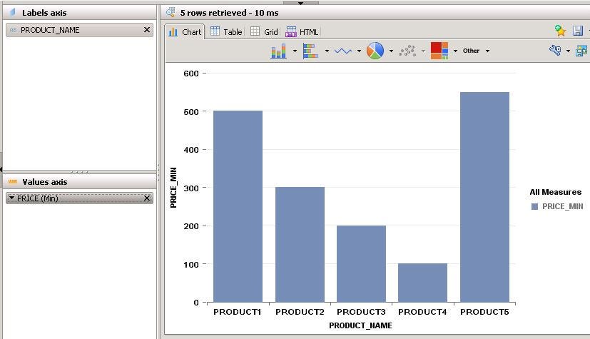
• Select the magnifying glass which says Data Preview. Select the option ‘Open the Data preview editor’. You will land up with the below screen.

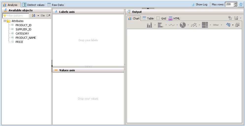
• We can see the output in different formats. Drag and drop the fields in value axis, which you want to see on the Y-axis and drag and drop the fields in the label axis which you want to see on X-axis.
• The output will be available in different formats such as Chart, Table, Grid, HTML.

• To view the output in a table format, select the Raw data option. This output is the join from two tables, namely PRODUCT and PRODUCT_DESC.

NOTE: Attribute views are not used for any reports, hence we will consume these views in the Analytic view.

Now, let’s start creating an Analytic View in SAP HANA.

Creating an Analytic View in SAP HANA

• As discussed earlier, for designing any views, we need SAP HANA Modeller Perspective. Further inside the Content section, choose the package name under which you want to create an Analytic view. Right-click on Package -> New -> Analytic view.

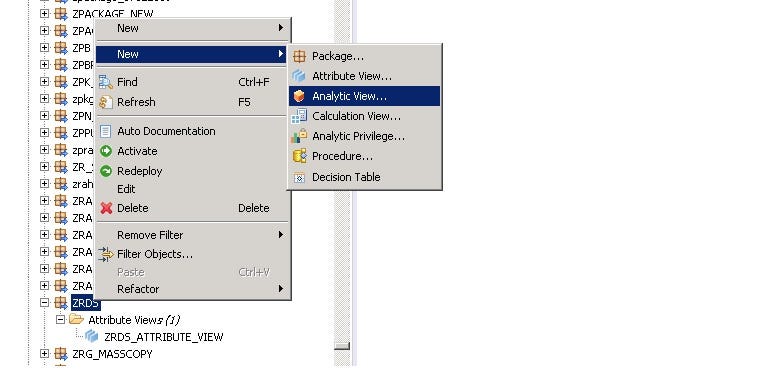
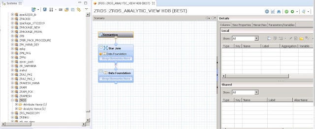
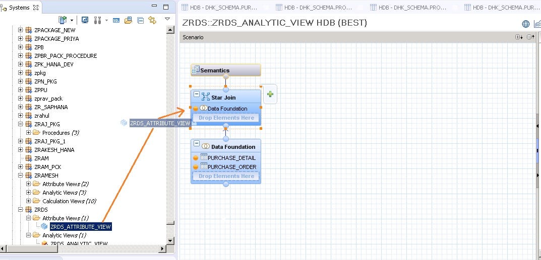
• Once you select the appropriate option, you will land to this screen of the Analytic view.
• Data foundation: We can add the dimensions and fact tables. Multiple tables can be added here.
• Star Join: We add the attribute views here which we have already created. This node creates join with the fact tables from the data foundation.

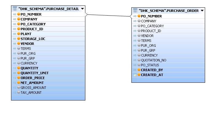
• Drag 2 tables namely ‘PURCHASE_DETAIL’ and ‘PURCHASE_ORDER’ from ‘DHK_SCHEMA’ and drop into the data foundation node.

NOTE: We can also add tables in the data foundation node with the plus sign located on the data foundation node when we hover the mouse.

• Further, select the fields from the Detail panel, which you want to use in the Analytic view. Also, join the field on which we want to perform joins. Here we have linked ‘PO_NUMER’ from both the tables.

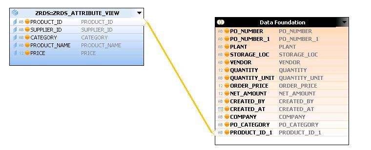
• Drag and drop the attribute view ‘ZRDS_ATTRIBUTE_VIEW’ (which we created in the last tutorial) inside Star Join.

• Again inside Detail panel, join the fields accordingly.

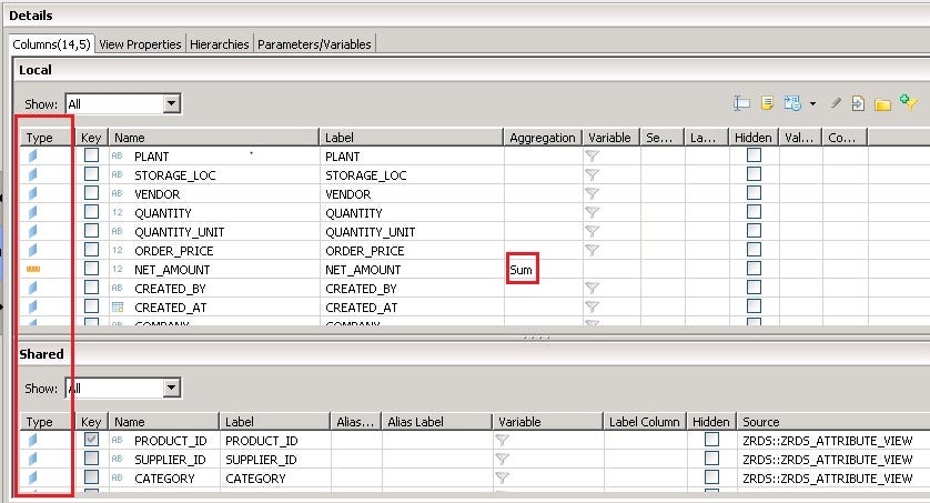
• Now, select the Semantics node. All the fields which we have selected will be listed. We need to mark the fields as an Attribute type or Measure type. This can be done manually or by auto-assign. Navigate towards the extreme right of the screen to find the icon of auto-assign. Blue color specifies Attribute type and orange color specifics the Measure type.

• Once, all the fields are marked with a specific type, save, activate, and hit the data preview icon.
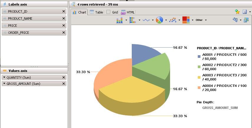
• Again, the same result screen will be displayed as in Attribute view. We have different formats to display in the Analysis tab. Drag and drop the fields in the label axis and value axis. Here, I have displayed the data in the pie chart format.

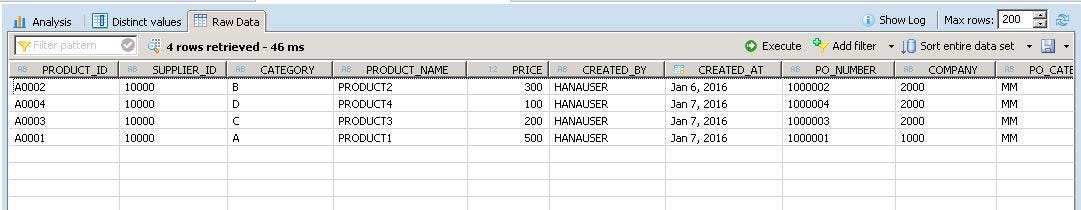
• In the Raw data tab, it will be displayed in the table format as shown below.

Now, let’s start creating a Calculation View in SAP HANA.

Creating a Calculation View in SAP HANA

Calculation view is a very powerful Information View. The drawback of the Analytic view is that it consists of only one fact table. To overcome this limitation, Calculation View came into the picture. It can consist of more than a fact table. The following are the steps to create a simple Calculation view.

• Navigate to the appropriate package. Choose the Calculation view.

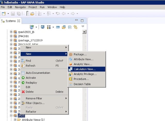
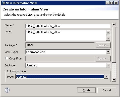
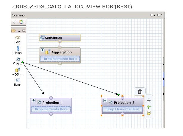
• As you know, the Calculation view is segregated into 2 parts: Graphical and SQL Script. Here we will take an example of Graphical Calculation View. Hit the Finish button.

Here, we have 5 different types of nodes:

• JOIN: This node connects two tables or two objects into a single object. The join types can be inner join, left outer join, right outer join, text join.

NOTE: We can connect only two objects to the JOIN node.

• UNION: This node performs a union between multiple sources.
• PROJECTION: This node is used to select the tables, filter the columns of the table. You can also select the analytic view which you created earlier. Besides, only one source object is used while working in the Projection node. If you wish to add more tables than create the separate projection nod for each table.
• AGGREGATION: In this node, you can perform aggregation on specific dimensions and measures.
• RANK: Ranking of values takes place here based on a criterion.

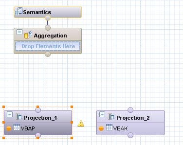
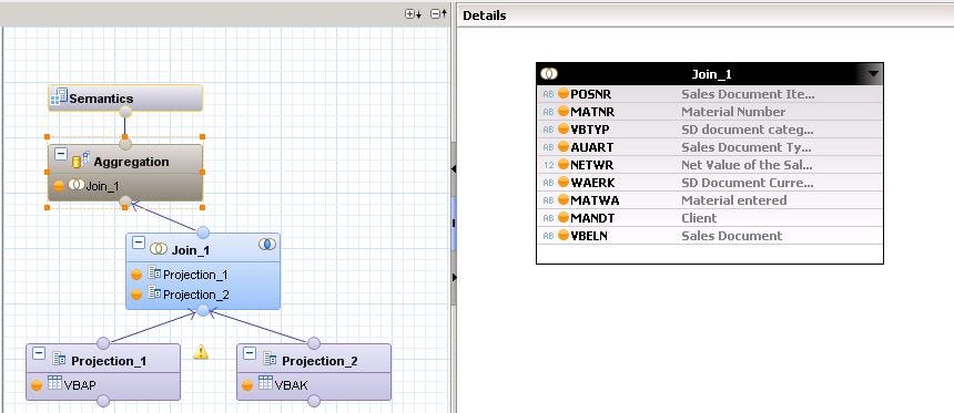
Drag and drop two projection nodes (one for VBAK and one for VBAP).

• Let us consider the standard SAP tables for our example. In the catalog tab, search for ECC2HANA_SD schema. We will do a join of two tables: VBAK (Sales Document: Header Data) and VBAP(Sales Document: Item Data).
• From the ‘VBAK’ table, I have selected fields such as MANDT, VBELN, VBTYP, AUART, NETWR, WAERK.
• From the ‘VBAP’ table, I have selected fields such as MANDT, VBELN, POSNR, MATNR, MATWA

• Further, drag and drop Join node. Connect the connectors of the Projection node to a connector of the Join node.

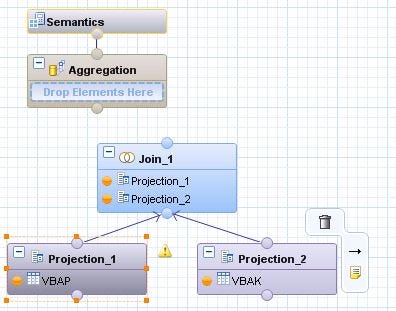
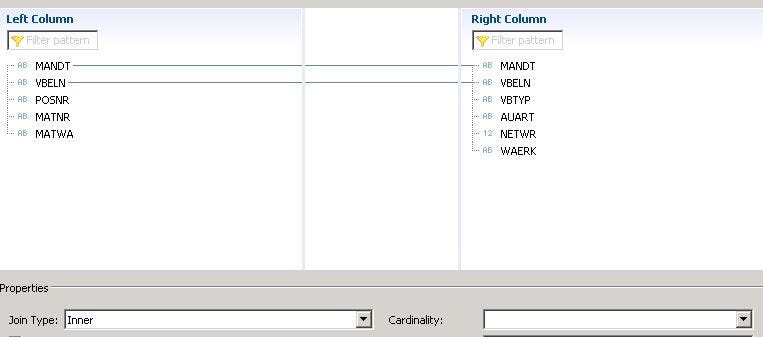
• Double click on the Join node and connect the fields on whom we want a join to be performed. Connect the fields which are common in both tables.

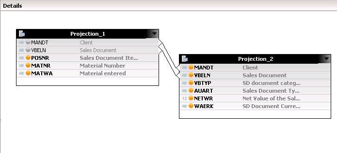
• Double click on the connection to change the join type if needed. I have changed the join type as ‘Inner’.

• Double click on the Aggregation node and select the fields which you want to see in the Calculation view. The bullets of the selected fields will change into orange color.

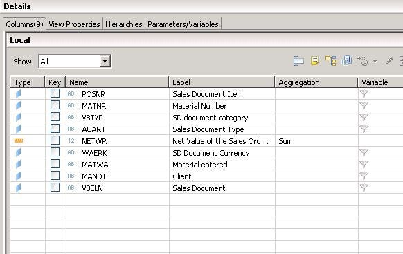
• Click on the Semantics node. You will get the display of all the fields which you want to see in the Calculation view. Mark the field type as either Attribute or Measure. You can also opt to hit the ‘Auto-assign icon’ located at the extreme right of the screen.

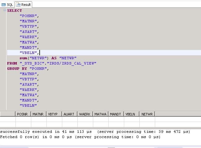
• Save, activate, and hit the data preview icon. This time I have selected the option of ‘Open in SQL Editor’. There are zero records fetched since the table had no entries.

The illustrations above will help individuals and professionals learn about the concepts of HANA Modeling in HANA.

---

Source (s):

SAP HANA Overview

Introduction to SAP HANA Modeling

Social Media Share :